CUDA Tips: nvcc’s -code, -arch, -gencode
Introduction People may feel confused by the options of -code, -arch, -gencode when compiling their CUDA codes. Although the official guidance explains the d...

My previous post, “Fused Operations in Tensorflow”, introduced the basics of operation fusion in deep learning by showing how to enable the grappler optimizer in Tensorflow to recognize the supported patterns and then fuse them together for better performance. In that post, I briefly talked about the Conv-Bias-Relu pattern, which is a great fit for fusion. In this post, by constrast, I will dive deeper into the Conv-Bias-Relu computation pattern and discuss why and how it can be fused.
Let’s start from the convolution shown in the following figure, which takes two parameters - a 3x3 input and a 2x2 weight - and outputs a 2x2 array.
Fig 0. Convolution's Computational Pattern
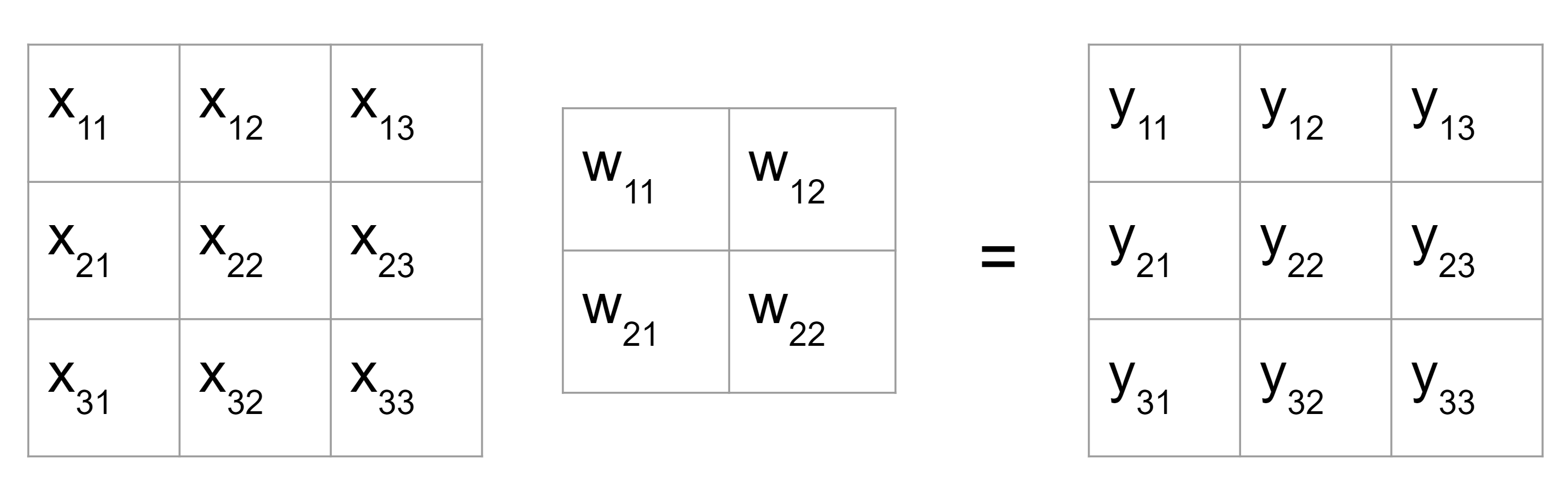
The convolution forward pass computes a weighted sum of the current input element as well as its surrounding neighbors. The process can be much easier to understand with the equations shown as below that match the above Fig. 0.
| Convolution equations |
|---|
| y11 = w11x11 + w12x12 + w21x21 + w22x22 |
| y12 = w11x12 + w12x13 + w21x22 + w22x23 |
| y21 = w11x21 + w12x22 + w21x31 + w22x32 |
| y22 = w11x22 + w12x23 + w21x32 + w22x33 |
Here w, x, and y are weight, input, and output arrays respectively. To get a
better sense of how the Tensorflow API does this, let’s have a look at a code
snippet of using tf.nn.conv2d to perform above computation. In the example, we
use the synthetic data for the x and w.
import tensorflow as tf
x = tf.reshape(tf.range(0, 9, dtype=tf.float32), (1, 3, 3, 1))
print("x:\n", x[0, :, :, 0].numpy())
w = tf.ones((2, 2, 1, 1))
print("w:\n", w[:, :, 0, 0].numpy())
y = tf.nn.conv2d(x, w, (1, 1), 'VALID', data_format='NHWC')
print("y:\n", y[0, :, :, 0].numpy())
x:
 [[0. 1. 2.]
  [3. 4. 5.]
  [6. 7. 8.]]
w:
 [[1. 1.]
  [1. 1.]]
y:
 [[ 8. 12.]
  [20. 24.]]
The convolution backward pass is to compute the gradients of w and x. Let’s suppose e is the error returned by any cost/loss function and thus the gradients of x and w are written as dw (= ∂e/∂w) and dx (= ∂e/∂x). According to the chain rule, we can easily get dw = ∂e/∂w = (∂e/∂y)(∂y/∂w) = dy⋅x. More precisely, the equations for dw are:
| Weight gradient equations |
|---|
| dw11 = dy11x11 + dy12x12 + dy21x21 + dy22x22 |
| dw12 = dy11x12 + dy12x13 + dy21x22 + dy22x23 |
| dw21 = dy11x21 + dy12x22 + dy21x31 + dy22x32 |
| dw22 = dy11x22 + dy12x23 + dy21x32 + dy22x33 |
In Tensorflow, tf.compat.v1.nn.conv2d_backprop_filter is used to calculate the
dw. It should be noted that though conv2d_backprop_filter is a separate API,
its computation pattern is essentially a convolutin but with the x as the input array
and dy as the weight array. Therefore, for learning purposes we can still call conv2d to realize its
functionality. The following script shows the results from
conv2d_backprop_filter can be matched with conv2d. In the test, the x is
synthetic data and we assume the dy is full of ones.
x = tf.reshape(tf.range(0, 9, dtype=tf.float32), (1, 3, 3, 1))
print("x:\n", x[0, :, :, 0].numpy())
dy = tf.ones((1, 2, 2, 1))
print("dy:\n", dy[0, :, :, 0].numpy())
dw = tf.compat.v1.nn.conv2d_backprop_filter(
    x, [2, 2, 1, 1], dy, [1, 1, 1, 1], 'VALID', use_cudnn_on_gpu=True,
    data_format='NHWC', dilations=[1, 1, 1, 1])
print("dw:\n", dw[:, :, 0, 0].numpy())
dy = tf.reshape(dy, (2, 2, 1, 1))
dw_copy = tf.nn.conv2d(x, dy, (1, 1), 'VALID', data_format='NHWC')
dw_copy = tf.reshape(dw_copy, (2, 2, 1, 1))
print("dw_equivalent:\n", dw_copy[:, :, 0, 0].numpy())
x:
 [[0. 1. 2.]
  [3. 4. 5.]
  [6. 7. 8.]]
dy:
 [[1. 1.]
  [1. 1.]]
dw:
 [[ 8. 12.]
  [20. 24.]]
dw_equivalent:
 [[ 8. 12.]
  [20. 24.]]
Similarly, the input gradients can be calculated by dx = ∂e/∂x = (∂e/∂y)(∂y/∂x) = dy⋅w. From the equations below, the computation pattern is actually still a convolution but the input and weight end up being the dy and a reversed w.
| Input gradient equations |
|---|
| dx11 = w11dy11 |
| dx12 = w12dy11 + w11dy12 |
| dx13 = w12dy12 |
| dx21 = w21dy11 + w11dy21 |
| dx22 = w22dy11 + w21dy12 + w12dy21 + w11dy22 |
| dx23 = w22dy12 + w12dy22 |
| dx31 = w21dy21 |
| dx32 = w22dy21 + w21dy22 |
| dx33 = w22dy22 |
In Tensorflow, we have tf.compat.v1.nn.conv2d_backprop_input to compute the
dx. In addition, to match its results, we can still use conv2d but need to pad
the dy and reverse the w before the call. The script shows this process with
synthetic data in w and all ones in dy.
dy = tf.ones((1, 2, 2, 1))
print("dy:\n", dy[0, :, :, 0].numpy())
w = tf.reshape(tf.range(0, 4, dtype=tf.float32), (2, 2, 1, 1))
print("w:\n", w[:, :, 0, 0].numpy())
dx = tf.compat.v1.nn.conv2d_backprop_input(
    (1, 3, 3, 1), filter=w, out_backprop=dy, strides=(1, 1, 1, 1),
    padding='VALID', use_cudnn_on_gpu=True, data_format='NHWC',
    dilations=[1, 1, 1, 1])
print("dx:\n", dx[0, :, :, 0].numpy())
dy = tf.pad(dy, [[0,0],[1,1],[1,1],[0,0]])
print("padded dy=\n", dy[0, :, :, 0].numpy())
w = tf.reverse(w, axis=[0, 1])
print("reversed w=\n", w[:, :, 0, 0].numpy())
dx_copy = tf.nn.conv2d(dy, w, (1, 1), 'VALID', data_format='NHWC')
print("dx_equivalent=\n", dx_copy[0, :, :, 0].numpy())
dy:
 [[1. 1.]
  [1. 1.]]
w:
 [[0. 1.]
  [2. 3.]]
dx:
 [[0. 1. 1.]
  [2. 6. 4.]
  [2. 5. 3.]]
padded dy=
 [[0. 0. 0. 0.]
  [0. 1. 1. 0.]
  [0. 1. 1. 0.]
  [0. 0. 0. 0.]]
reversed w=
 [[3. 2.]
  [1. 0.]]
dx_equivalent=
 [[0. 1. 1.]
  [2. 6. 4.]
  [2. 5. 3.]]
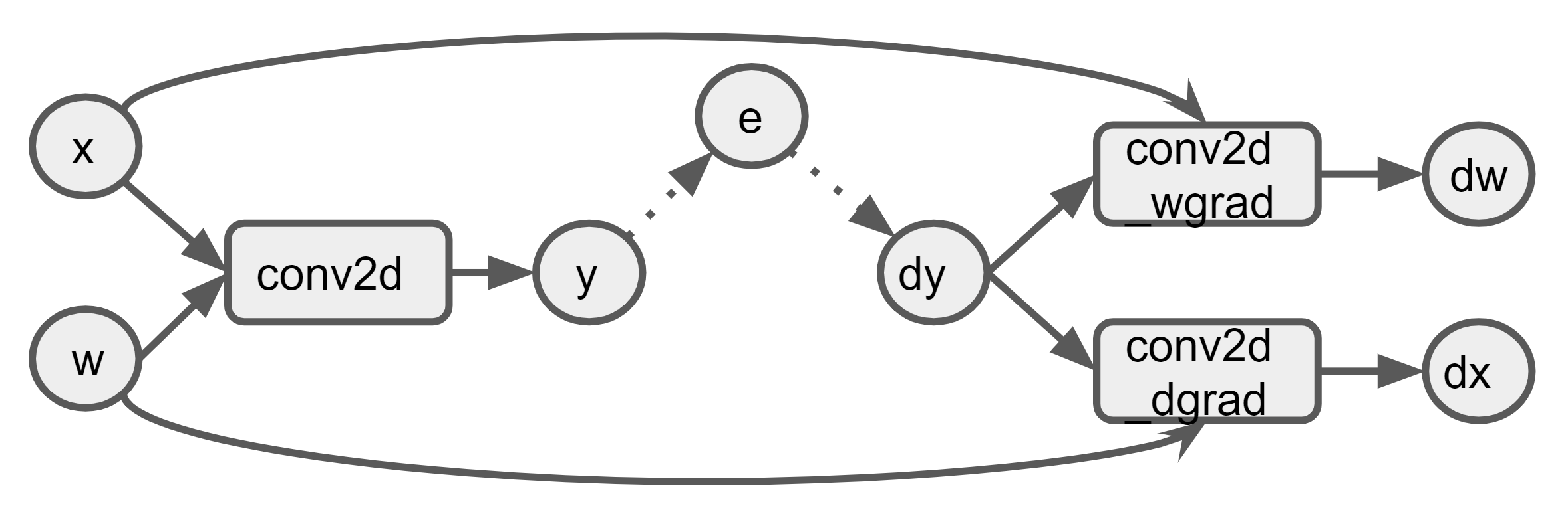
If we put all the input/output tensors and operation nodes into one graph, we can see the data flow and dependencies more clearly. The takeaway here is that the input x and w for the forward pass is still needed in backward convolution to compute dw and dx respectively. In other words, both the input x and w need to be alive even when the forward pass has already done. Whereas, the output y from the forward convolution will no longer be used in backward pass.
Fig 1. Convolution
Compared to the convolution, the bias add is much simpler. The following equation shows that we add the input x with the bias b to obtain y.
| BiasAdd equations |
|---|
| y = x + b |
Since the bias b is a trainable parameter, we use the following equations to get the db as well as dx, which are essentially a forward operation of dy.
| Bias/Input gradient equations |
|---|
| db = ∂e/∂b = (∂e/∂y)(∂y/∂b) = dy |
| dx = ∂e/∂x = (∂e/∂y)(∂y/∂x) = dy |
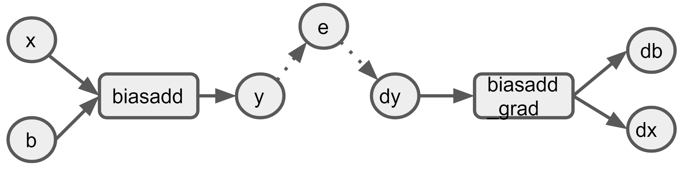
The figure below shows the bias add operations. Apparently, neither of the input nor the output from the forward pass is needed in the backward pass.
Fig 2. BiasAdd
The ReLU is also straightforward. From the equation below, we can learn that there is no trainable parameters and we only have one input x and one output y.
| ReLU equations |
|---|
| y = 0, x ≤ 0 |
| y = x, x > 0 |
The backward pass only need to compute the dx, and to do so we can use x or y. Mathematically, they are same but using y would be more “fusion-friendly”, which will be explained later.
| Input gradient equations |
|---|
| dx = 0, y ≤ 0 (or x ≤ 0) |
| dx = dy, y > 0 (or x > 0) |
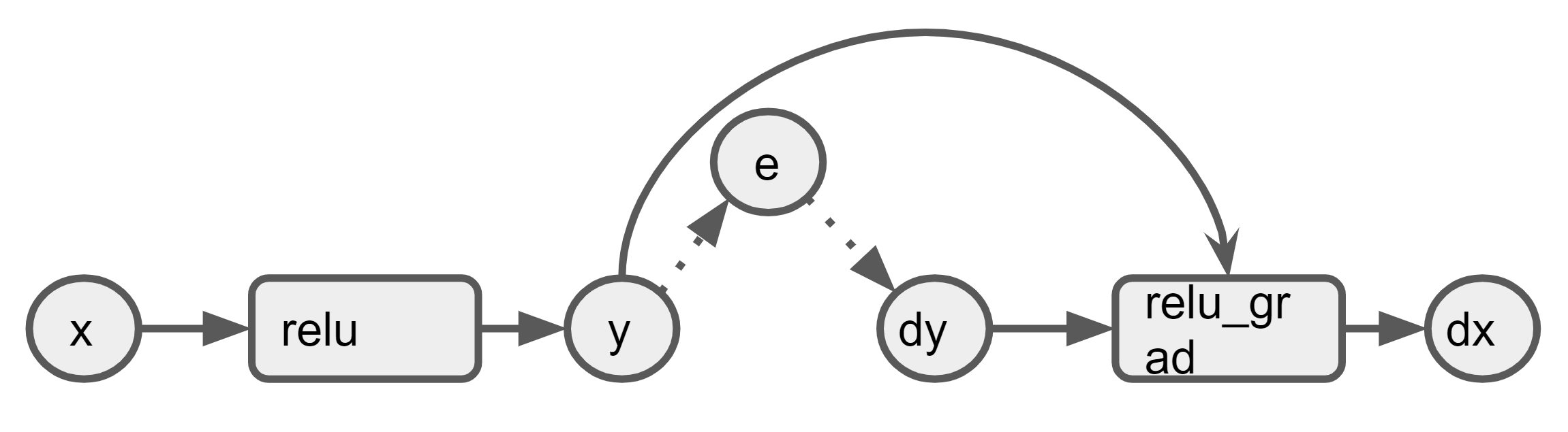
After we put all nodes in a graph, we can observe the backward pass only needs the output from the forward pass.
Fig 3. ReLU
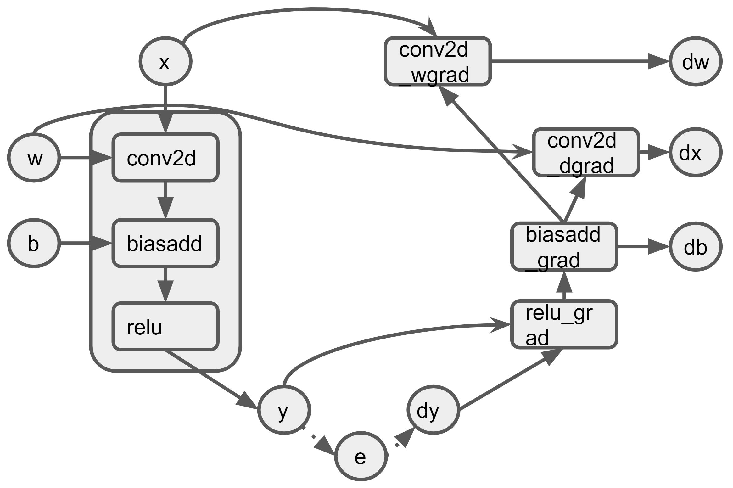
Now, we can draw all these three operations together in one figure. Based on the above analysis, the Conv-Bias-Relu can be safely fused into one operation since the backward pass won’t use any intemediate results from the fused operation but only its input x, w and its output y.
Fig 4. Fused Ops
It is worth to mention that this post focuses mainly on the scenario of training and discusses the fusion from the perspective of the data dependencies. In reality, the decision to fuse will be more complex than it seems.
Introduction People may feel confused by the options of -code, -arch, -gencode when compiling their CUDA codes. Although the official guidance explains the d...
When training neural networks with the Keras API, we care about the data types and computation types since they are relevant to the convergence (numeric stab...
Introduction This post focuses on the GELU activation and showcases a debugging tool I created to visualize the TF op graphs. The Gaussian Error Linear Unit,...
Introduction My previous post, “Demystifying the Conv-Bias-ReLU Fusion”, has introduced a common fusion pattern in deep learning models. This post, on the ot...
Introduction Recently, I am working on a project regarding sparse tensors in Tensorflow. Sparse tensors are used to represent tensors with many zeros. To sav...
Introduction On my previous post Inside Normalizations of Tensorflow we discussed three common normalizations used in deep learning. They have in common a tw...
Introduction Recently I was working on a project related to the operation fusion in Tensorflow. My previous posts have covered several topics, such as how to...
Introduction My previous post, “Fused Operations in Tensorflow”, introduced the basics of operation fusion in deep learning by showing how to enable the grap...
Introduction The computations in deep learning models are usually represented by a graph. Typically, operations in the graph are executed one by one, and eac...
Introduction Horovod is an open source toolkit for distributed deep learning when the models’ size and data consumption are too large. Horovod exhibits many ...
Introduction Recurrent Neural Network (RNN) is widely used in AI applications of handwriting recognition, speech recognition, etc. It essentially consists of...
Introduction Recently I came across with optimizing the normalization layers in Tensorflow. Most online articles are talking about the mathematical definitio...