Moving Mean and Moving Variance In Batch Normalization

Introduction

On my previous post Inside Normalizations of Tensorflow we discussed three common normalizations used in deep learning. They have in common a two-step computation: (1) statistics computation to get mean and variance and (2) normalization with scale and shift, though each step requires different shape/axis for different normalization types. Among them, the batch normalization might be the most special one, where the statistics computation is performed across batches. More importantly, it works differently during training and inference. While working on its backend optimization, I frequently encountered various concepts regarding mean and variance: moving mean, batch mean, estimated mean, and even saved mean to name a few. Therefore, this post will look into the differences of these terms and show you how they are used in deep learning framework, Tensorflow Keras Layers, and deep learning library, CUDNN Batch Norm APIs.

Typical Batch Norm

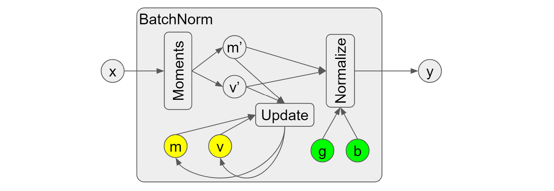
In a typical batch norm, the “Moments” op will be first called to compute the statistics of the input x, i.e. the batch mean/variance (or current mean/variance, new mean/variance, etc.). It reflects the local information of x. As shown in Figure 1, we use m' and v' to represent them. After statistics computation, they are fed into the “Update” op to obtain the new moving mean/variance (or running mean/variance). The formula used here is moving_* = moving_* ⋅ momentum + batch_* ⋅ (1 - momentum) where the momentum is a hyperparameter. (Instead, CUDNN uses a so called exponential average factor and thus its updating formula becomes moving_* = moving_* ⋅(1 - factor) + batch_* ⋅factor.) In the second step for normalization, the “Normalize” op will take the batch mean/variance m' and v' as well as the scale (g) and offset (b) to generate the output y.

Figure 1. Typical batch norm in Tensorflow Keras

The following script shows an example to mimic one training step of a single batch norm layer. Tensorflow Keras API allows us to peek the moving mean/variance but not the batch mean/variance. For illustrative purposes, I inserted codes to the Keras python APIs to print out the batch mean/variance. Note, the moving mean/variance are not trainable variables so that they cannot be updated during the backpropagation. For this reason, we skip the backward pass in the training step.

bn = tf.keras.layers.BatchNormalization(momentum=0.5,
    beta_initializer='zeros', gamma_initializer='ones',
    moving_mean_initializer='ones', moving_variance_initializer='ones',
    fused=False)
# Training Step 0 (skip the real scale/offset update)
x0 = tf.random.uniform((2,1,2,3))
print("x(step0):", x0.numpy())

y0 = bn(x0, training=True)
print("moving_mean(step0): ", bn.moving_mean.numpy())
print("moving_var(step0): ", bn.moving_variance.numpy())
print("y(step0):", y0.numpy())

The outputs of the above code are pasted below and we can see that the moving mean/variance are different from the batch mean/variance. Since we set the momentum to 0.5 and the initial moving mean/variance to ones, the updated mean/variance are calculated by moving_* = 0.5 + 0.5 ⋅batch_*. On the other hand, it can be confirmed that the y_step0 is computed with the batch mean/variance through (x_step0 - batch_mean) / sqrt(batch_var + 0.001)

x(step0):
[[[[0.16513085 0.9014813  0.6309742 ]
   [0.4345461  0.29193902 0.64250207]]]
 [[[0.9757855  0.43509948 0.6601019 ]
   [0.60489583 0.6366315  0.6144488 ]]]]
!!! batch_mean:
   [0.5450896  0.5662878  0.63700676]
!!! batch_var: 
   [0.08641606 0.05244513 0.00027721]
moving_mean(step0):
   [0.7725448 0.7831439 0.8185034]
moving_var(step0):
   [0.543208   0.5262226  0.50013864]
y(step0):
[[[[-1.2851115   1.4499114  -0.16879845]
   [-0.37388456 -1.186722    0.15376663]]]
 [[[ 1.4567168  -0.5674678   0.6462345 ]
   [ 0.20227909  0.30427837 -0.6312027 ]]]]

To make it closer to real settings, we conduct one more training step with another input x and these are the moving mean/variance we can get:

moving_mean(step1):
    [0.72269297 0.63172865 0.62922215]
moving_var(step1):
    [0.29549128 0.28121024 0.25281417]

At last, we mimic one step of inference as below. In the script, we rename the moving mean/variance to estimized mean/variance, which represents the accumulated and frozen moving mean/variance from the training stage.

# Inference Step
x_infer = tf.random.uniform((2,1,2,3))
print("x(infer):", x_infer.numpy())

y_infer = bn(x_infer, training=False)
print("estimated_mean(infer): ", bn.moving_mean.numpy())
print("estimated_var(infer): ", bn.moving_variance.numpy())
print("y(infer):", y_infer.numpy())

From the outputs below, it is easy to verify that y_infer is computed with the estimated mean/variance rather than batch mean/variance: (x_infer - estimated_mean) / sqrt(estimated_var + 0.001). Besides, we can see that the estimated mean/variance equals to the moving mean/variance from the above step1, indicating they are no longer updated in inference stages. To sum up, the takeaway here is that the batch norm will keep accumulating batch mean/variance into the moving mean/variance during training, which will be evolved into frozen estimated mean/variance to be used during inference.

x(infer):
[[[[0.8292774  0.634228   0.5147276 ]
   [0.39108086 0.5809028  0.04848182]]]
 [[[0.1776321  0.70470166 0.49190843]
   [0.3460425  0.5079107  0.2216742 ]]]]
estimated_mean(infer):
   [0.72269297 0.63172865 0.62922215]
estimated_var(infer):
   [0.29549128 0.28121024 0.25281417]
y(infer):
[[[[ 0.1957438   0.00470471 -0.22726214]
   [-0.60901    -0.09567499 -1.1527207 ]]]
 [[[-1.0010114   0.13736498 -0.2725562 ]
   [-0.69172347 -0.2330758  -0.8089484 ]]]]

The complete python script is here.

Fused Batch Norm

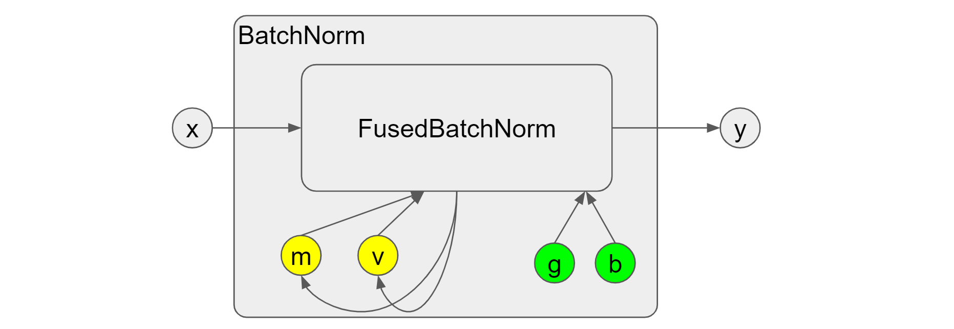
In the above example we explictly turned off the operation fusion by setting fused=False of the Keras BatchNormalization layer. In practice, however, we usually set it to None (to use fusion whenever possible) or True (to force the fusion) for better speedup. Figure 2 shows what the fused operation looks like in batch norm. There is only one big op FusedBatchNorm and its inputs/outputs are consistent with the combined “Moments” + “Update” + “Normalize” ops in Figure 1. Whereas there is no simple way to get the batch mean/variance m' and v', which will pose a bigger challenge for the synchronized batch norm that we will talk about later. In addition, it is worth to mention that we can’t assume the bitwise equality of the outputs from the fused op and non-fused ops.

Figure 2. Fused batch norm on GPUs

Batch Norm Backpropagation

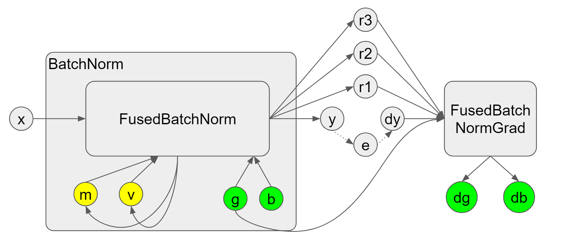
The backend of the FusedBatchNorm relies on the CUDNN library for GPUs, which introduces another terms: saved mean and inverse variance. As shown in Figure 3, we depict a forward and backward pass of batch norm using the fused ops. The following script reflects these two passes. From the figure, we notice that the FusedBatchNormGrad requires dy and g (scale) (whose mathematical basis can be found here) as well as r1, r2, and r3. In fact, r1 and r2 are the saved mean and inverse variance respectively, which are computed from the batch mean and variance. They are produced and cached during the forward pass and then used in the backward pass to avoid the overhead of re-compute. To sum up, the saved mean and inverse variance are designed out of consideration for performance in the batch norm backpropagation using CUDNN.

Figure 3. Fused batch norm and backpropagation

bn = tf.keras.layers.BatchNormalization(momentum=0.5,
    beta_initializer='zeros', gamma_initializer='ones',
    moving_mean_initializer='ones', moving_variance_initializer='ones',
    fused=True)
x0 = tf.random.uniform((2,1,2,3))
with tf.GradientTape() as t:
  t.watch(x0)
  y0 = bn(x0, training=True)
  loss = tf.reduce_sum(y0)
grads = t.gradient(loss, [x0, bn.trainable_variables])

The saved mean and saved inverse variance (r1 and r2) are usually hidden from users in Tensorflow. However, we can still peek the contents by explicitly using the ops defined in tf.raw_ops. The following script shows the code.

y, moving_mean, moving_var, r1, r2, r3 = tf.raw_ops.FusedBatchNormV3(
    x=x, scale=scale, offset=offset, mean=mean, variance=variance,
    epsilon=0.001, exponential_avg_factor=0.5, data_format='NHWC',
    is_training=True, name=None)
print("moving_mean:", moving_mean.numpy())
print("moving_var:", moving_var.numpy())
print("saved mean:", r1.numpy())
print("saved inv var:", r2.numpy())

By feeding the op with the same inputs used in the above exmaple, we can print the corresponding moving mean/variance and r1/r2 for comparison. The moving mean/variance are same with the results from the 0th step of the above example (They are not exactly equivalent because we use fused op here.). Additionally, we can observe that r1 is essentially the batch mean, while r2 is calculated by 1 / sqrt(batch_var + 0.001).

moving_mean: [0.7725448 0.7831439 0.8185034]
moving_var: [0.5576107  0.5349634  0.50018483]
saved mean: [0.5450896  0.5662878  0.63700676]
saved inv var: [ 3.3822396  4.325596  27.981367 ]

The complete python script for the batch norm backpropagation is here. The script to use tf.raw_ops is here. Besides, I prepared a CUDA sample to directly call CUDNN library with the same inputs as the above example. From there we can test that the saved mean/inv variance are not required parameters.

Synchronized Batch Norm

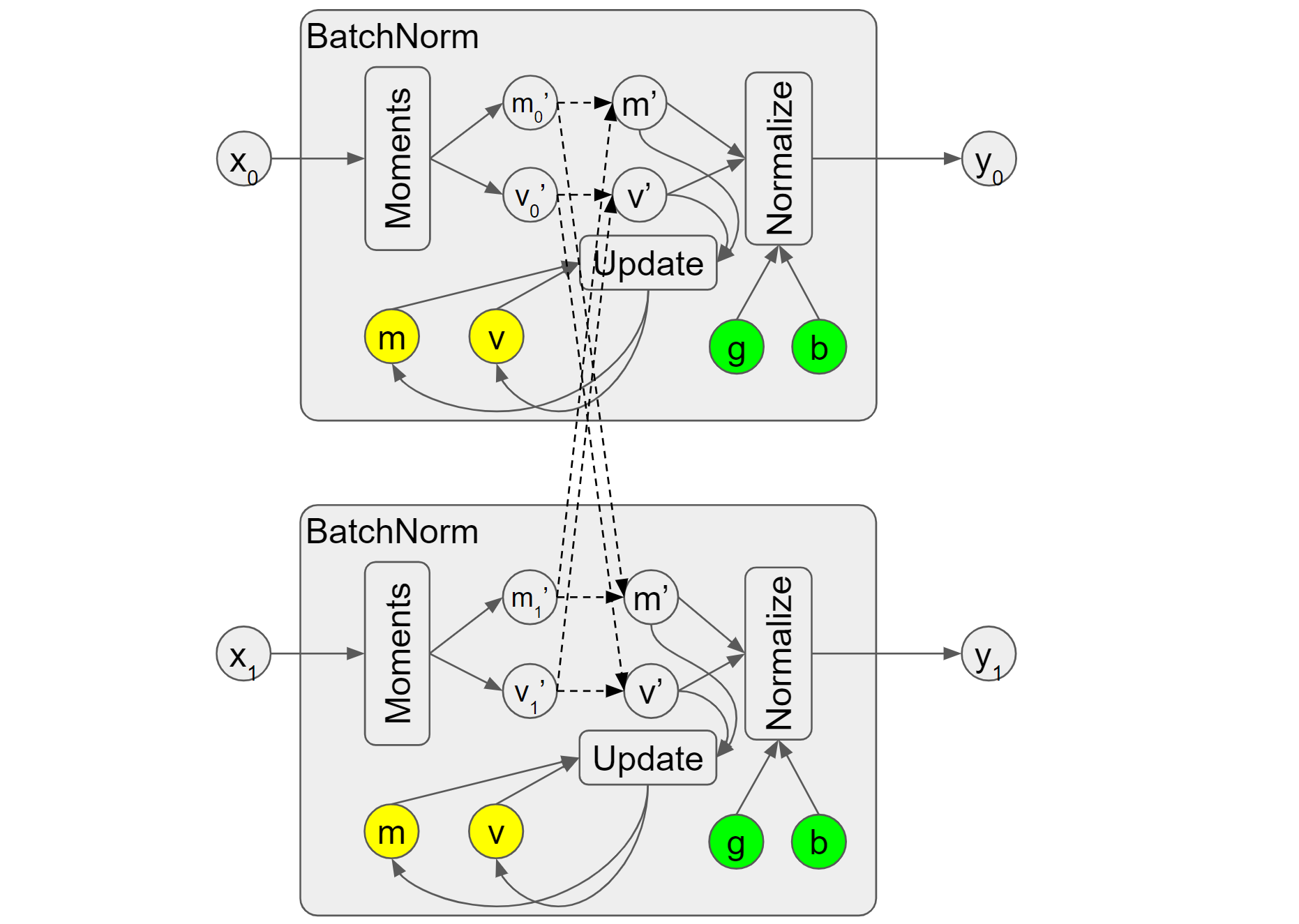
Lastly, I would like to briefly talk about the synchronized batch norm, which are preferrable when performing distributed training and the batch size are too small for each compute node. In that case (e.g., the object detection tasks), we can use synchronized batch norm to get better statistics by considering samples from different nodes. Here I will use the implementation from the horovod: hvd.SyncBatchNormalization. It overrides the “Moments” op to conduct communication among nodes and return the group mean and variance, which reflect the mean and variance of samples from all participant nodes. In Figure 4, they are denoted as m' and v'. Subsequently, “Update” will take them to update the moving group mean/variance, and “Normalize” will also take them to compute the outputs. As we mentioned previously, the fused op doesn’t expose the batch mean/variance and thus it will be challenging to do the communication to get the group mean/variance and therefore synchronized batch norm only support non-fused ops.

Figure 4. Synchronized batch norm

The following script shows how to use the hvd.SyncBatchNormalization. We intentionally set the different inputs x0 for different ranks.

# Make sure that different ranks have different inputs.
tf.random.set_seed(hvd.local_rank())
x0 = tf.random.uniform((2,1,2,3))

sync_bn = hvd.SyncBatchNormalization(axis=-1, momentum=0.5,
    beta_initializer='zeros', gamma_initializer='ones',
    moving_mean_initializer='ones', moving_variance_initializer='ones')
print("moving_mean: ", sync_bn.moving_mean.numpy())
print("moving_var: ", sync_bn.moving_variance.numpy())

When running with horovodrun -np 2 python tf_hvd_bn_sync.py, we can get the outputs below, where the batch mean/variance are actually already group mean/variance after the communication and the moving mean/variance are computed based on them.

[1,0]:!!! batch_mean:[0.45652372 0.5745423  0.65629953]
[1,1]:!!! batch_mean:[0.45652372 0.5745423  0.65629953]
[1,0]:!!! batch_var:[0.0657616  0.0710133  0.00523123]
[1,1]:!!! batch_var:[0.0657616  0.0710133  0.00523123]
[1,0]:moving_mean:[0.7282618  0.78727114 0.8281498 ]
[1,1]:moving_mean:[0.7282618  0.78727114 0.8281498 ]
[1,0]:moving_var:[0.5328808  0.53550667 0.50261563]
[1,1]:moving_var:[0.5328808  0.53550667 0.50261563]

Note, the dot lines showing the communication in Figure 4 might not precisely depict what happens under the hood. The group mean is simply the average of batch means from different ranks that can be done through an allreduce communication; however, the group variance needs a new round of computation with the updated group mean rather than communication: (x - group_mean) ^ 2 / (N⋅batch_size), where N is number of ranks.

The complete python script is here.

Reference

• Tensorflow Batch Normalization API
• Deriving the Gradient for the Backward Pass of Batch Normalization
• CUDNN Batch Normalization API
• Add SyncBatchNormalization layer for TensorFlow

• 2022 3
• 2021 8
• 2020 1